Application to noise correlation functions

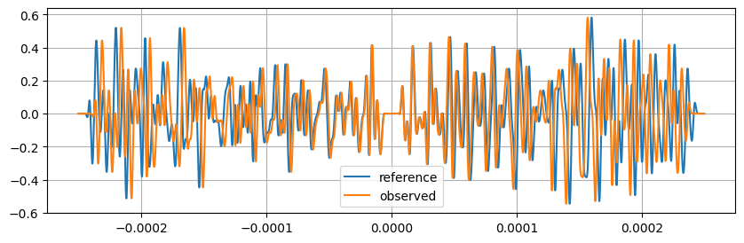
A test to show that the stretcher works exactly the same way for positive/negative times

Thus the same approch can be used for two-sided correlation functions.

See jupyter notbook named “examples” for details.

import time
import numpy as np
import matplotlib.pyplot as plt

from scipy.signal.windows import tukey
from scipy.signal import butter, sosfiltfilt

from coodddaaaa.stretching import Stretcher # This package
from coodddaaaa.utils import Timer, polyspace, TukeyWindow # This package

dt = 1e-7  # sampling, sec
nt = int(5e-4 // dt)   # number of samples in time
t0 = -2.5e-4   # start time in sec

time_array = t0 + np.arange(nt) * dt  # seconds  (NEVER use np.linspace for time vectors)
fnyquist = 0.5 / dt    # Hz

tmin = 0.1e-4   # begin of time window in sec
tmax = 2.4e-4   # end of time window in sec
fmin = 0.01 * fnyquist   # lower freq Hz
fmax = 0.05 * fnyquist   # upper freq Hz

eps_true = 0.02  # the imposed stretching coeff

# create the time taper
tukeywin = TukeyWindow(tmin-0.01*nt*dt, tmin, tmax, tmax+0.01*nt*dt)
taper = tukeywin(time_array) + tukeywin(-time_array)

# and the bandpass filter
sos = butter(4.0, [fmin / fnyquist, fmax / fnyquist], output="sos", btype="band")  # for
bandpass = lambda signal_array: sosfiltfilt(sos, signal_array)  # predefined bandpass filter

# Build the reference band-pass / tapered coda
y_reference = bandpass(np.random.randn(nt)) * taper

# Build the observed signal, a stretched version of it + noise
stretcher0 = Stretcher(t0=t0, nt=nt, dt=dt, eps=np.array([eps_true]), norm=False)  # for stretching only
y_observed = stretcher0.stretch(y_reference)[0, :]  # only one trace here

# Display
plt.figure(figsize=(10, 3))
plt.plot(time_array, y_reference, label="reference")
plt.plot(time_array, y_observed, label="observed");
plt.gca().legend();
plt.gca().grid(True)